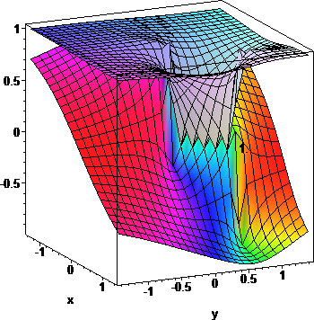
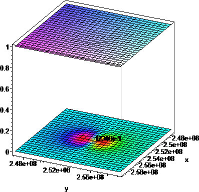
Earth-Moon unit-distance system geodesics (cyan) and gravitational pool (purple/blue). Masses are indicated relative to ME=1
The N-body problem is the problem of finding how N-masses interact gravitationally. Although it has no closed form solution, the solution can be approximated using Maple.
To understand the problem better, we solve first the reduced 3-body problem, which is the same problem with N=3 and some of the masses being stationary. A fairly good exercise for the mechanics of this problem, is to simulate sending a probe to the Moon from Earth. In this case we have 2 stationary bodies (Earth and Moon) and we seek the calculational details which will allow us to put the probe in lunar orbit.
Let's assume that our probe has a mass of 1000 tons. The whole procedure consists of three subproblems:
The first step is covered in most standard ballistics texts. The next three steps require a fairly more elaborate understanding.
Geodesics
First we need to understand the geodesics of gravitational attraction around the system[1]. Once we have the geodesics of the system, we can visualize the gravitational pool that's created around the Earth and Moon system. The geodesics are given by Newton's Law of Universal Gravitation (NLUG).
Earth Orbit
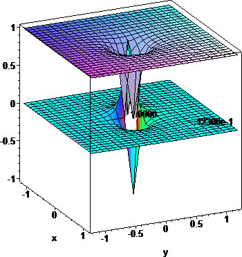
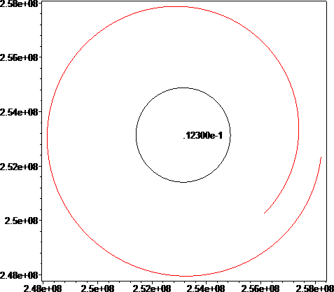
The geodesics which characterize a 1000 ton probe in medium orbit are shown:
To put the probe in Earth orbit, we find a velocity which keeps it roughly on an elliptical orbit. For this we choose an altitude and try to find a velocity which keeps it in orbit. For our example, we choose an altitude of ae=6000 km, which gives a medium orbit. For such an orbit, a velocity u=2.85 km/sec suffices:
Lunar Orbit
The geodesics which characterize a 1000 ton probe in lunar orbit are shown:
To put the probe in Lunar orbit, we again choose a desired altitude and a velocity which keeps the probe in orbit. For our example, we choose an altitude of am=1200 km, in which case a velocity u=0.8 km/sec suffices:
Earth-Moon Trajectory
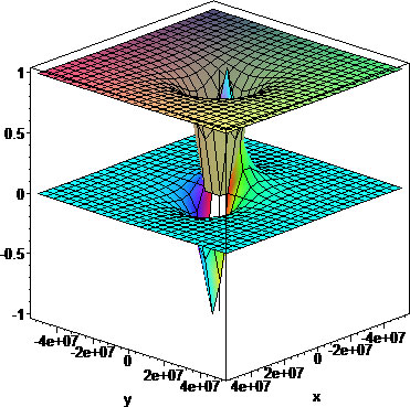
The geodesics which characterize a 1000 ton probe thrown towards the Moon are shown:
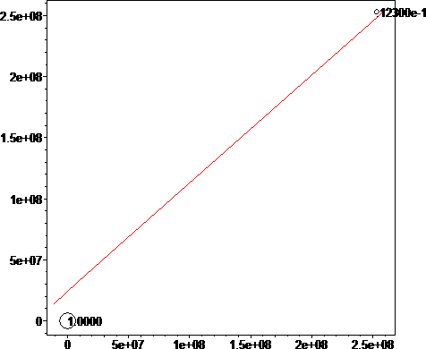
The in between trajectory can be calculated now. After one full revolution from the Earth orbit, we fire our thrusters and give the probe some appropriate velocity to send it to the moon. How do we calculate the appropriate velocity to give to the probe? Let's assume that our starting location is at θ=-3*π/4 around Earth and we need to reach the destination position -3*π/4 around the moon. We would reach this position if we started with an escape velocity ve equal to infinity. Because we can't do that, we need to reduce the velocity ve to ve', one which will bring us am-close to the moon, where am is the moon altitude of the lunar orbit we need to go into. After testing drag and some trial and error, we find that an escape velocity of ve~14.18 km/sec is sufficient[2].
Now if we combine the three steps in the correct order, we can simulate Apollo 11's travel to the moon[3][4].
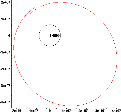
A different more distant orbit for the reduced 3-body problem is shown below:
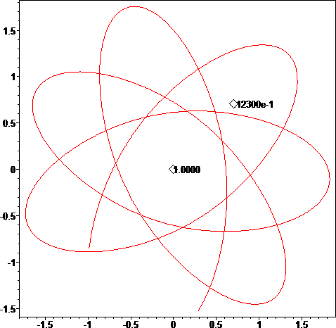
An animated version of the above orbit is shown below:
The General N-body Problem
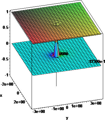
The general N-body problem involves finding all trajectories of N interacting masses, under the influence of their own gravity as a function of time. For this, one sums all forces involved and allows a minimum dt which determines the new positions of all masses. It is a bit tricky to figure out the velocities of the masses so that the system is in a stable state, but can be done.
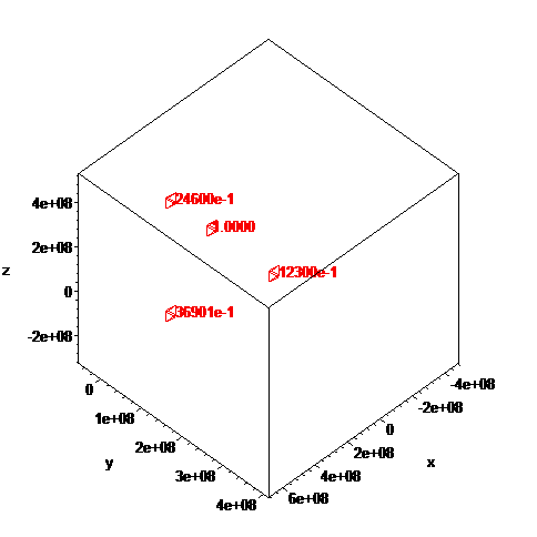
An example is given on the figure above, which shows the partial trajectory for 4 masses under the influence of gravity, an Earth and three moons, one with mass equal to Earth's Moon and two more moons with masses 2 and 3 times that of Earth's moon, with all masses approximately in orbit around the Earth mass[5].
Note the vertical lines where the space-time continuum tears because of gravity. These tears tend to create a 2d singularity in space-time.